"Graph Function" Dialog

How can I access information on this dialog?

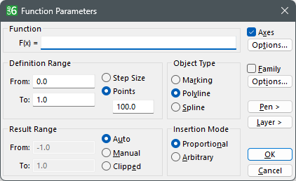
After selecting the command Draw > Function Plotter > Create Graph the above shown dialog window "Function Parameters" appears. Here the function term is entered, the definition range is set and the object type for the generated function is selected. The function term must include the variable x. A multi-variable function also requires the second variable a. To generate a multi-variable function the option "Family" must be active. The text display in the function edit field changes accordingly from F(x) to F(x,a).

The defined basic functions are listed further below. To simplify editing omit the multiplication operator * between a number and a variable.

Example

35*x can be entered as 35x

3*x*a can be entered as 3xa

To generate a graph it is necessary to define a range on the X-axis. This range is called the definition range. This range can exist of up to 1999 points. The user can either edit the number of desired points (setting "Points"), or define the distance between two points (setting "Step Size"). Depending on the size of the definition range the amount of points needed is calculated automatically.

For every x-value from the definition range the resulting values are calculated. The program can find the maximum and minimum value in the resulting range itself. The Y-axis is scaled accordingly. This is achieved by activating the radio button "Auto".

If the resulting Y-range exceeds 200 times the definition range it is necessary to switch to the setting "Clipped". This can be important when a function contains undefined points, pole points or extreme values. If the setting "Clipped" is active all values that exceed the range are ignored and not used for the display of the graph.

If the setting "Manual" is active the values defined in the field "From" and "To" are used to calculate the resulting range of the graph. If a value exceeds the area for the resulting range it is taken automatically.

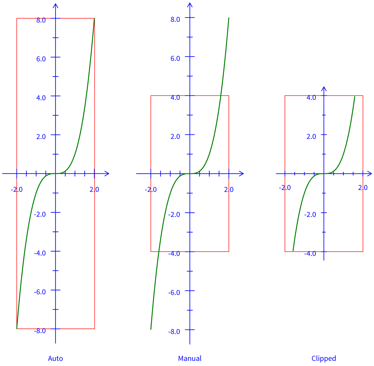
In the following picture the three different insertion modes are presented. The graph shows the function F(x)=x^3 in the definition range from -2 to 2. The area displayed in red is the rectangle entered by the user. The resulting range is always -4 to 4. If "Auto" is active this range is calculated by the program. If the setting "Manual" is active the complete resulting range is used to display the graph. The setting "Clipped" cuts the graph at the borders of the defined range.

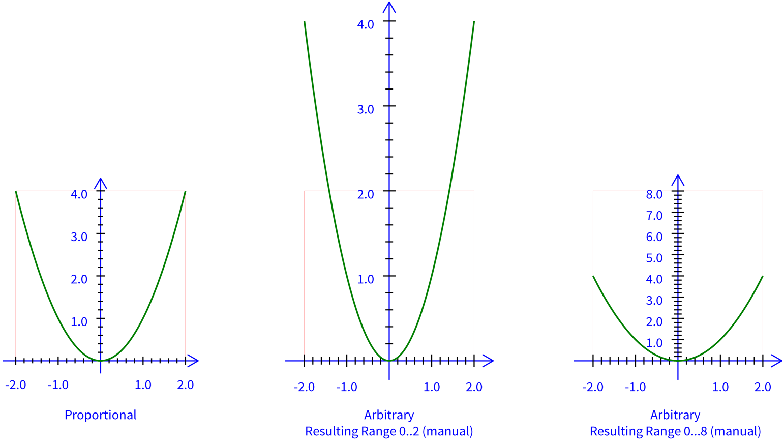
The selected insertion mode defines whether a unit on the X-axis equals one unit on the Y-axis. If the user wants these units to be the same the mode "Proportional" has to be chosen. If independent unit sizes for the axis are needed the mode "Arbitrary" is recommended. The red frame displays the rectangle, the user defines where to insert the graph.

To define a specific relation between X-axis values and Y-axis values it is recommended to set the resulting range mode to "Manual". The relation can easily be entered by using the grid, snap functions, direct entry and the orthogonal mode. See next picture:

In the example the function F(x)=x^2 is displayed with the mode "Proportional". To be able to compare the values the second corner point of the rectangle is entered with the direct entry and relative coordinates ( e.g: w=50 h=50). The resulting area is displayed in red in the example shown. To double the scale of the Y-axis in the right picture switch to the mode "Manual" and define the resulting range from 0 to 2. The second corner point is entered again with relative coordinates (w=50 h=50). The third example is generated the same way except the resulting range is extended from 0 to 8.

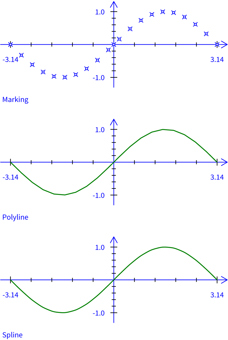
The user can select the object type for the graph. It can be either a polyline, a spline or simple markings. Markings are inserted at the calculated base points. The spline curve allows to generate a smooth graph with few base points.

Caution: The smoothness of a spline curve is not based on mathematical precision of the entered function. Spline curves are built of the same base points like a polyline or markings. The resulting smoothness is a part of the mathematical way the spline curve is calculated and has no relationship to the way the entered function is defined!

It is highly recommended not to use the spline curve when the function is not constant. For example the absolute function (ABS( )) at the point 0.

To add axis and texts to the graph activate the option "Axis". The "Option"-button below allows the user to specify the additional parameters in the "Graph Axes" dialog. More details can be found in the description of this dialog window.

To generate a multi-variable function plot the user has to activate the option "Family". A multi-variable function needs the additional parameter a beside variable x. The parameter is set to the next defined value after each completed calculation for the variable x in the definition range. This value is used to calculate a new graph with the updated a value. Up to 100 parameters are allowed. So up to 100 function graphs can be generated. The values for the parameter a can be edited in the "Graph Family" dialog. The dialog field is opened with the "Option"-button below the checkbox "a-Parameters". More details can be found in the description of this dialog window.

The following operators and functions are supported:

Standard operators:

+

Plus

-

Minus

*

Multiplication

/

Division

^

Power

Trigonometric functions:

SIN( )

Sine Function

COS( )

Cosine Function

TAN( )

Tangent Function

COT( )

Cotangent Function

SINH( )

Hyperbolic Sine Function

COSH( )

Hyperbolic Cosine Function

TANH( )

Hyperbolic Tangent Function

COTH( )

Hyperbolic Cotangent Function

ASIN( )

Arc Sine Function

ACOS( )

Arc Cosine Function

ATAN( )

Arc Tangent Function

ACOT( )

Arc Cotangent Function

ASINH( )

Hyperbolic Arc Sine Function

ACOSH( )

Hyperbolic Arc Cosine Function

ATANH( )

Hyperbolic Arc Tangent Function

ACOTH( )

Hyperbolic Arc Cotangent Function

Additional functions:

ABS( )

Absolute Function

SQRT( )

Square root Function

LN( )

Natural Logarithm (to the base of e)

LOG( )

Logarithm to the base of 10

EXP( )

Exponential Function

SIGN( )

Sign Function

FAC( )

Factorial